Tutorial : Fitting a line profile using Monte Carlo Markov Chains
In this tutorial you will, hopefully, learn how fit Lyman-alpha line profiles using a Monte Carlo Markov Chain with zELDA. The MCMC engine is emcee (https://emcee.readthedocs.io/en/stable/).
Getting started
Let’s start by loading zELDA creating a mock line profile that we will fit later. For more details on how to create a mock line profile go to Mock line profiles
>>> import Lya_zelda as Lya
>>> your_grids_location = '/This/Folder/Contains/The/Grids/'
>>> Lya.funcs.Data_location = your_grids_location

>>> Geometry = 'Thin_Shell_Cont'
>>> LyaRT_Grid = Lya.load_Grid_Line( Geometry )

>>> # Defining the model parameters:
>>> z_t      = 0.5   # redshift of the source
>>> V_t      = 40.0  # Outflow expansion velocity [km/s]
>>> log_N_t  = 20.   # Logarithmic of the neutral hydrogen column density [cm**-2]
>>> t_t      = 0.01  # Dust optical depth
>>> log_EW_t = 1.5   # Logarithmic the intrinsic equivalent width [A]
>>> W_t      = 0.5   # Intrinsic width of the line [A]
>>> F_t      = 1.    # Total flux of the line

>>> # Defining the quality of the line profile:
>>> PNR_t  = 15.0 # Signal to noise ratio of the maximum of the line.
>>> FWHM_t = 0.2  # Full width half maximum diluting the line. Mimics finite resolution. [A]
>>> PIX_t  = 0.1  # Wavelength binning of the line. [A]

>>> w_Arr , f_Arr , s_Arr = Lya.Generate_a_real_line( z_t , V_t, log_N_t, t_t, F_t, log_EW_t, W_t , PNR_t, FWHM_t, PIX_t, LyaRT_Grid, Geometry )
where /This/Folder/Contains/The/Grids/ is the place where you store the LyaRT data grids, as shown in the installation section. And… It’s done! w_Arr is a numpy array that contains the wavelength where the line profile is evaluated. Meanwhile, f_Arr is the actual line profile. s_Arr is the uncertainty of the flux density. Remeber that if you want to use the line profile grid with lower RAM memory occupation you must pass MODE=’LIGHT’ to Lya.load_Grid_Line.
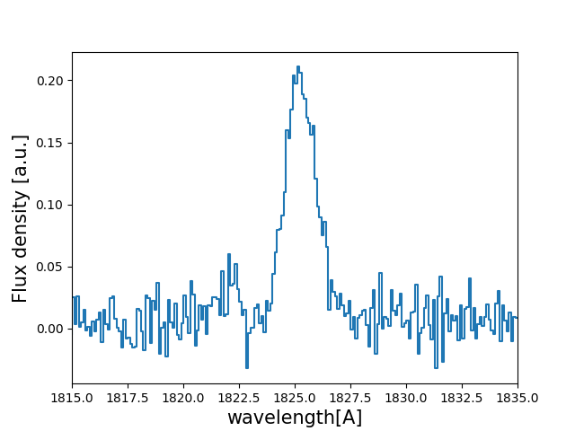
Let’s have a look to how the line looks:
>>> w_Arr , f_Arr , s_Arr  = Lya.Generate_a_real_line( z_t , V_t, log_N_t, t_t, F_t, log_EW_t, W_t , PNR_t, FWHM_t, PIX_t, LyaRT_Grid, Geometry )

>>> w_pix_Arr , f_pix_Arr = Lya.plot_a_rebinned_line( w_Arr , f_Arr , PIX_t )

>>> import pylab as plt
>>> plt.plot( w_pix_Arr , f_pix_Arr )
>>> plt.xlabel('wavelength[A]' , size=15 )
>>> plt.ylabel('Flux density [a.u.]' , size=15 )
>>> plt.xlim(1815,1835)
>>> plt.show()
The MCMC anlysis
Let’s now set the configuration for the MCMC analysis.
>>> N_walkers = 200 # Number of walkers
>>> N_burn    = 200 # Number of steps to burn-in
>>> N_steps   = 300 # Number of steps to run after burning-in
Now let’s choose the method to initialize the walkers. There are basically two methods: using the deep neural network or doing a fast particle swarm optimization (PSO). For this tutorial we will use the deep neural network.
>>> MODE = 'DNN'
If you want to use instead the PSO you can set MODE = ‘PSO’.
Now let’s get the regions where we want to originally spawn our lovely walkers:
>>> log_V_in , log_N_in , log_t_in , log_E_in , W_in , z_in , Best = Lya.MCMC_get_region_6D( MODE , w_Arr , f_Arr , s_Arr , FWHM_t , PIX_t , LyaRT_Grid , Geometry )
The variables log_V_in, log_N_in, log_t_in, log_E_in, W_in and z_in are python lists of two elements containing the range where to spawn the walkers for the logarithmic of the bulk velocity, the logarithmic of the HI column density, the logarithmic of the dust optical, the logarithmic of the intrinsic equivalent width, the intrinsic width of the line and the redshift. For example, z_in[0] contains the minimum redshift and z_in[0] the maximum. Actually this step is not necessary and if you want you can continue without defining these variables or setting them as you please. Also, remember that these list only maker where the walkers are spawned. They might actually get outside this volume if the best fitting region is outside.
Let’s now run the MCMC:
>>> sampler = Lya.MCMC_Analysis_sampler_5( w_Arr , f_Arr , s_Arr , FWHM_t , N_walkers , N_burn , N_steps , Geometry , LyaRT_Grid , z_in=z_in , log_V_in=log_V_in , log_N_in=log_N_in , log_t_in=log_t_in , log_E_in=log_E_in , W_in=W_in )
sampler is an object of the python package emcee. Note that there is a way of forcing the redshift to be inside z_in. We decided to this with only this property in case you know the redshift of the source before hand. you can do this by passing FORCE_z=True to Lya.MCMC_Analysis_sampler_5.
Now let’s get the actual value of the predicted properties and their 1-sigma uncertainty. For this, in this tutorial we chose as our prediction the percentile 50th o the probability distribution function of the variables. For the +-1-sigma uncertainty we choose the percentiles 16th and 84th.
>>> Q_Arr = [ 16 , 50 , 84 ] # You can add more percentiles here, like 95

>>> perc_matrix_sol , flat_samples = Lya.get_solutions_from_sampler( sampler , N_walkers , N_burn , N_steps , Q_Arr )
flat_samples contains the MCMC chains flatten. perc_matrix_sol is a 2-D array with dimensions 6xlen(Q_Arr) containing the percentiles of the variables. You can extract the values doing something like:
>>> # redshift.
>>> z_16     =     perc_matrix_sol[ 3 , 0 ] # corresponds to Q_Arr[0]
>>> z_50     =     perc_matrix_sol[ 3 , 1 ] # corresponds to Q_Arr[1]
>>> z_84     =     perc_matrix_sol[ 3 , 2 ] # corresponds to Q_Arr[2]

>>> # Expansion velocity.
>>> V_16     = 10**perc_matrix_sol[ 0 , 0 ]
>>> V_50     = 10**perc_matrix_sol[ 0 , 1 ]
>>> V_84     = 10**perc_matrix_sol[ 0 , 2 ]

>>> # dust optical depth.
>>> t_16     = 10**perc_matrix_sol[ 2 , 0 ]
>>> t_50     = 10**perc_matrix_sol[ 2 , 1 ]
>>> t_84     = 10**perc_matrix_sol[ 2 , 2 ]

>>> # Intrinsic width.
>>> W_16     =     perc_matrix_sol[ 5 , 0 ]
>>> W_50     =     perc_matrix_sol[ 5 , 1 ]
>>> W_84     =     perc_matrix_sol[ 5 , 2 ]

>>> # Logarithmic of the intrinsic equivalent width.
>>> log_E_16 =     perc_matrix_sol[ 4 , 0 ]
>>> log_E_50 =     perc_matrix_sol[ 4 , 1 ]
>>> log_E_84 =     perc_matrix_sol[ 4 , 2 ]

>>> # Logarithmic of the HI column density.
>>> log_N_16 =     perc_matrix_sol[ 1 , 0 ]
>>> log_N_50 =     perc_matrix_sol[ 1 , 1 ]
>>> log_N_84 =     perc_matrix_sol[ 1 , 2 ]
Let’s compare the MCMC prediction with the actual input:
>>> print( 'The true redshift                 is' , z_t      , 'and the predicted is' , z_50     , '(-' , z_50-z_16         , ', +' , z_84-z_50         , ')' )
>>> print( 'The true expansion velocity       is' , V_t      , 'and the predicted is' , V_50     , '(-' , V_50-V_16         , ', +' , V_84-V_50         , ')' )
>>> print( 'The true dust optical depth       is' , t_t      , 'and the predicted is' , t_50     , '(-' , t_50-t_16         , ', +' , t_84-t_50         , ')' )
>>> print( 'The true intrinsic width          is' , W_t      , 'and the predicted is' , W_50     , '(-' , W_50-W_16         , ', +' , W_84-W_50         , ')' )
>>> print( 'The true log of HI column density is' , log_N_t  , 'and the predicted is' , log_N_50 , '(-' , log_N_50-log_N_16 , ', +' , log_N_84-log_N_50 , ')' )
>>> print( 'The true log of equivalent width  is' , log_EW_t , 'and the predicted is' , log_E_50 , '(-' , log_E_50-log_E_16 , ', +' , log_E_84-log_E_50 , ')' )
which should look something like:
The true redshift                 is 0.5 and the predicted is 0.49991074547548753 (- 1.9665578543492934e-05 , + 0.0014991528312225944 )
The true expansion velocity       is 40.0 and the predicted is 30.741297629627855 (- 1.097915986182759 , + 244.88872432354253 )
The true dust optical depth       is 0.01 and the predicted is 0.04392859929402969 (- 0.035550939281926146 , + 0.0103076912398413 )
The true intrinsic width          is 0.5 and the predicted is 0.2859470609607235 (- 0.09765211992507192 , + 0.06363668998672473 )
The true log of HI column density is 20.0 and the predicted is 20.215438954615962 (- 2.4584647794744434 , + 0.027551697514507367 )
The true log of equivalent width  is 1.5 and the predicted is 1.7365288817793056 (- 0.29375812799042955 , + 0.033311663274792735 )
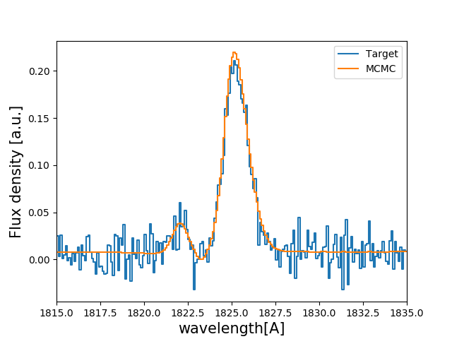
Now let’s plot the lines and see how they compare:
>>> # Infinite signal to noise in the model
>>> PNR = 100000.

>>> # Compute line
>>> w_One_Arr , f_One_Arr , _  = Lya.Generate_a_real_line( z_50, V_50, log_N_50, t_50, F_t, log_E_50, W_50, PNR, FWHM_t, PIX_t, LyaRT_Grid, Geometry )

>>> # Make cooler
>>> w_pix_One_Arr , f_pix_One_Arr = Lya.plot_a_rebinned_line( w_One_Arr , f_One_Arr , PIX_t )

>>> # Plot
>>> plt.plot( w_pix_Arr     , f_pix_Arr     , label='Target' )
>>> plt.plot( w_pix_One_Arr , f_pix_One_Arr , label='MCMC'   )
>>>
>>> plt.legend(loc=0)
>>> plt.xlabel('wavelength[A]' , size=15 )
>>> plt.ylabel('Flux density [a.u.]' , size=15 )
>>> plt.xlim(1815,1835)
>>> plt.show()
This should give you something like this:
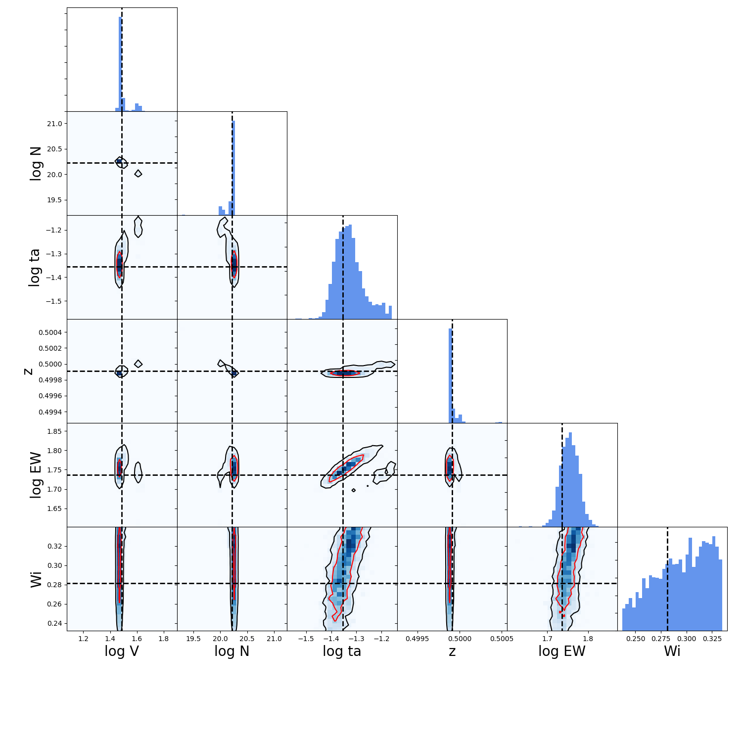
Now let’s do a correlation plot to see where the walkers are. For this we will use the function make_corner_plots which is define just below in this same page, in Tool to make corraltion plots .
>>> make_corner_plots( flat_samples )
>>> plt.show()
And it should give you something like:
And.. with that it’s done. Now you know how to use the MCMC implementation in zELDA.
Tool to make corraltion plots
This is just a code to plot the walkers and the probability distribution funtions of the posteriors of the MCMC analysis.
def make_corner_plots( my_chains_matrix ):

    import numpy as np
    import pylab as plt

    N_dim = 6

    ax_list = []

    label_list = [ 'log V' , 'log N' , 'log ta' , 'z' , 'log EW', 'Wi'  ]

    MAIN_VALUE_mean   = np.zeros(N_dim)
    MAIN_VALUE_median = np.zeros(N_dim)
    MAIN_VALUE_MAX    = np.zeros(N_dim)

    for i in range( 0 , N_dim ):

        x_prop = my_chains_matrix[ : , i ]

        x_prop_min = np.percentile( x_prop , 10 )
        x_prop_50  = np.percentile( x_prop , 50 )
        x_prop_max = np.percentile( x_prop , 90 )

        x_min = x_prop_50 - ( x_prop_max - x_prop_min ) * 1.00
        x_max = x_prop_50 + ( x_prop_max - x_prop_min ) * 1.00

        mamamask = ( x_prop > x_min ) * ( x_prop < x_max )

        MAIN_VALUE_mean[  i] = np.mean(       x_prop[ mamamask ] )
        MAIN_VALUE_median[i] = np.percentile( x_prop[ mamamask ] , 50 )

        HH , edges_HH = np.histogram( x_prop[ mamamask ] , 30 , range=[ x_prop_min , x_prop_max ] )

    plt.figure( figsize=(15,15) )

    Q_top = 80
    Q_low = 20

    for i in range( 0 , N_dim ):

        y_prop = my_chains_matrix[ : , i ]

        y_prop_min = np.percentile( y_prop , Q_low )
        y_prop_50  = np.percentile( y_prop , 50 )
        y_prop_max = np.percentile( y_prop , Q_top  )

        mask_y = ( y_prop > y_prop_min ) * ( y_prop < y_prop_max )

        y_min = y_prop_50 - np.std( y_prop[ mask_y ] )
        y_max = y_prop_50 + np.std( y_prop[ mask_y ] )

        for j in range( 0 , N_dim ):

            if i < j : continue

            x_prop = my_chains_matrix[ : , j ]

            x_prop_min = np.percentile( x_prop , Q_low )
            x_prop_50  = np.percentile( x_prop , 50 )
            x_prop_max = np.percentile( x_prop , Q_top )

            mask_x = ( x_prop > x_prop_min ) * ( x_prop < x_prop_max )

            x_min = x_prop_50 - np.std( x_prop[ mask_x ] )
            x_max = x_prop_50 + np.std( x_prop[ mask_x ] )

            ax = plt.subplot2grid( ( N_dim , N_dim ) , (i, j)  )

            ax_list += [ ax ]

            DDX = x_max - x_min
            DDY = y_max - y_min

            if i==j :

                H , edges = np.histogram( x_prop , 30 , range=[x_min,x_max] )

                ax.hist( x_prop , 30 , range=[x_min,x_max] , color='cornflowerblue' )

                ax.plot( [ MAIN_VALUE_median[i] , MAIN_VALUE_median[i] ] , [ 0.0 , 1e10 ] , 'k--' , lw=2 )

                ax.set_ylim( 0 , 1.1 * np.amax(H) )

            else :

                XX_min = x_min - DDX * 0.2
                XX_max = x_max + DDX * 0.2

                YY_min = y_min - DDY * 0.2
                YY_max = y_max + DDY * 0.2

                H , edges_y , edges_x = np.histogram2d( x_prop , y_prop , 30 , range=[[XX_min , XX_max],[YY_min , YY_max]] )

                y_centers = 0.5 * ( edges_y[1:] + edges_y[:-1] )
                x_centers = 0.5 * ( edges_x[1:] + edges_x[:-1] )

                H_min = np.amin( H )
                H_max = np.amax( H )

                N_bins = 10000

                H_Arr = np.linspace( H_min , H_max , N_bins )[::-1]

                fact_up_Arr = np.zeros( N_bins )

                TOTAL_H = np.sum( H )

                for iii in range( 0 , N_bins ):

                    mask = H > H_Arr[iii]

                    fact_up_Arr[iii] = np.sum( H[ mask ] ) / TOTAL_H

                H_value_68 = np.interp( 0.680 , fact_up_Arr , H_Arr )
                H_value_95 = np.interp( 0.950 , fact_up_Arr , H_Arr )

                ax.pcolormesh( edges_y , edges_x , H.T , cmap='Blues' )

                ax.contour( y_centers, x_centers , H.T , colors='k' , levels=[ H_value_95 ] )
                ax.contour( y_centers, x_centers , H.T , colors='r' , levels=[ H_value_68 ] )

                X_VALUE =  MAIN_VALUE_median[j]
                Y_VALUE =  MAIN_VALUE_median[i]

                ax.plot( [ X_VALUE , X_VALUE ] , [    -100 ,     100 ] , 'k--' , lw=2 )
                ax.plot( [    -100 ,     100 ] , [ Y_VALUE , Y_VALUE ] , 'k--' , lw=2 )

                ax.set_ylim( y_min-0.05*DDY , y_max+0.05*DDY )

            ax.set_xlim( x_min-0.05*DDX , x_max+0.05*DDX )

            if i==N_dim-1:
                ax.set_xlabel( label_list[j] , size=20 )

            if j==0 and i!=0 :
                ax.set_ylabel( label_list[i] , size=20 )

            if j!=0:
                plt.setp( ax.get_yticklabels(), visible=False)

            if j==0 and i==0:
                plt.setp( ax.get_yticklabels(), visible=False)

            if i!=len( label_list)-1 :
                plt.setp( ax.get_xticklabels(), visible=False)

    plt.subplots_adjust( left = 0.09 , bottom = 0.15 , right = 0.98 , top = 0.99 , wspace=0., hspace=0.)

    return None